
Background
This is the fifth article in the “Learn PyTorch by Examples” series. In the fourth article “Learn PyTorch by Example (4): Sequence Prediction with Recurrent Neural Networks (I)”, we introduced the sequence prediction problem and how to use a simple Recurrent Neural Network (RNN) to predict the sine function. In this article, we will go further and introduce two other commonly used neural networks for sequence prediction: Gated Recurrent Unit (GRU) and Long Short-Term Memory (LSTM).
The code for this article can be found in the T05_series_rnn folder in my GitHub repository https://github.com/jin-li/pytorch-tutorial.
Problems with RNN and Solutions
In the fourth article, we introduced the basic concepts and working principles of Recurrent Neural Networks (RNNs). RNN is a type of neural network that can handle sequence data, and it saves the previous data information at each time step, so it can handle sequence data. However, RNN also has some problems, such as the vanishing gradient and exploding gradient problems. The vanishing gradient and exploding gradient are common problems in deep learning, and they can cause the model to fail to converge or converge very slowly.
The vanishing gradient and exploding gradient are common problems in deep learning. In the backpropagation algorithm, the gradient is calculated using the chain rule:
$D_n = \sigma^{’}(z_1) w_1 \cdot \sigma^{’}(z_2) w_2 \cdot \ldots \cdot \sigma^{’}(z_{n-1}) w_{n-1} \cdot \sigma^{’}(z_n) w_n$
where $D_n$ is the gradient of the $n$-th layer, $\sigma^{’}(z_i)$ is the derivative of the activation function of the $i$-th layer, and $w_i$ is the weight of the $i$-th layer. It can be seen that the gradient is calculated by multiplying the derivative of the activation function and the weight of each layer. If the derivative of the activation function is less than 1, the gradient will decrease exponentially with the increase of the number of layers, leading to the vanishing gradient; if the derivative of the activation function is greater than 1, the gradient will increase exponentially with the increase of the number of layers, leading to the exploding gradient.
Long Short-Term Memory (LSTM) and Gated Recurrent Unit (GRU) are proposed to solve the vanishing gradient and exploding gradient problems in RNN. They control the flow of information by introducing gate mechanisms to solve the long-term dependency problem in RNN.
Introduction to LSTM and GRU
LSTM and GRU both introduce gate mechanisms to control the flow of information. The so-called gate mechanism multiplies the data by a coefficient between 0 and 1 to control whether to pass the data and how much data to pass, and this coefficient is calculated by a sigmoid activation function.
The difference between LSTM and GRU is that LSTM has three gates: Forget Gate, Input Gate, and Output Gate, while GRU has only two gates: Reset Gate and Update Gate. GRU has fewer parameters and less computation than LSTM, but LSTM generally performs better than GRU.
Long Short-Term Memory (LSTM)
Long Short-Term Memory (LSTM) is a type of gated recurrent neural network proposed by Hochreiter and Schmidhuber in 1997. LSTM introduces three gates: Forget Gate, Input Gate, and Output Gate to control the flow of information, thus solving the long-term dependency problem in RNN.
The structure of LSTM is shown in the following figure:
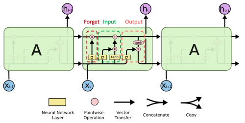
The derivation of the specific calculation formulas for the Forget Gate, Input Gate, and Output Gate is not given here. Interested readers can refer to this article Understanding LSTM Networks. Here we simply introduce the working principle of LSTM:
We assume that the memory data in LSTM is $C_t$, the hidden state is $h_t$, the input data is $x_t$, the Forget Gate is $f_t$, the Input Gate is $i_t$, and the Output Gate is $o_t$. The working principle of LSTM is as follows:
-
Forget Gate: The input of the Forget Gate is the input data $x_t$ at the current time step and the hidden state $h_{t-1}$ at the previous time step. The output of these two inputs after passing through the sigmoid function is a coefficient $f_t$ between 0 and 1. $f_t$ determines how much data from the previous time step needs to be retained. If $f_t$ is close to 0, the data from the previous time step will be forgotten; if $f_t$ is close to 1, the data from the previous time step will be retained.
-
Input Gate: The input of the Input Gate is the input data $x_t$ at the current time step and the hidden state $h_{t-1}$ at the previous time step. The output of these two inputs after passing through the sigmoid function is a coefficient $i_t$ between 0 and 1. $i_t$ determines how much data from the current time step needs to be retained. If $i_t$ is close to 0, the data from the current time step will be ignored; if $i_t$ is close to 1, the data from the current time step will be retained.
-
Update Memory: The formula for updating the memory is $C_t = f_t \cdot C_{t-1} + i_t \cdot \tilde{C}t$, where $\tilde{C}t$ is the output of the input data $x_t$ at the current time step and the hidden state $h{t-1}$ at the previous time step after passing through the tanh function. $C_t$ is the memory data at the current time step, $f_t \cdot C{t-1}$ is the memory data at the previous time step, and $i_t\cdot\tilde{C}_t$ is the input data at the current time step.
-
Output Gate: The input of the Output Gate is the input data $x_t$ at the current time step and the hidden state $h_{t-1}$ at the previous time step. The output of these two inputs after passing through the sigmoid function is a coefficient $o_t$ between 0 and 1. $o_t$ determines how much output data $h_t$ at the current time step needs to be retained. If $o_t$ is close to 0, the output data at the current time step will be ignored; if $o_t$ is close to 1, the output data at the current time step will be retained.
Gated Recurrent Unit (GRU)
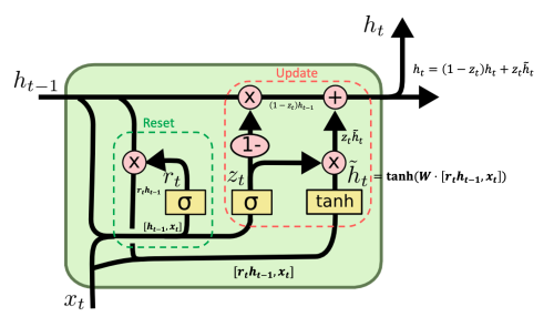
The Gated Recurrent Unit (GRU) is a simplified version of LSTM proposed by Cho et al. in 2014. GRU has only two gates: Reset Gate and Update Gate. Compared to LSTM, GRU has fewer parameters and less computation. Although LSTM generally performs better, GRU is also popular due to its simplicity.
The Reset Gate and Update Gate in GRU are actually simplified versions of the three gates in LSTM. The derivation of the specific calculation formulas is not given here. Interested readers can refer to this article Understanding LSTM Networks. Here we simply introduce the working principle of GRU:
We assume that the memory data in GRU is $h_t$, the input data is $x_t$, the Reset Gate is $r_t$, and the Update Gate is $z_t$. The working principle of GRU is as follows:
-
Reset Gate: The input of the Reset Gate is the input data $x_t$ at the current time step and the hidden state $h_{t-1}$ at the previous time step. The output of these two inputs after passing through the sigmoid function is a coefficient $r_t$ between 0 and 1. $r_t$ determines how much data from the previous time step needs to be retained. If $r_t$ is close to 0, the data from the previous time step will be ignored; if $r_t$ is close to 1, the data from the previous time step will be retained.
-
Update Memory: The formula for updating the memory is $\tilde{h}t = \tanh(W [r_t h{t-1}, x_t]) = \tanh(W_{xh} x_t + r_t \odot W_{hh} h_{t-1})$, where $\odot$ is element-wise multiplication. $\tilde{h}t$ is the memory data at the current time step, $W{xh} x_t$ is the input data at the current time step, and $r_t \odot W_{hh} h_{t-1}$ is the hidden state at the previous time step.
-
Update Gate: The input of the Update Gate is the input data $x_t$ at the current time step and the hidden state $h_{t-1}$ at the previous time step. The output of these two inputs after passing through the sigmoid function is a coefficient $z_t$ between 0 and 1. $z_t$ determines how much memory data at the current time step needs to be retained. If $z_t$ is close to 0, the memory data at the current time step will be ignored; if $z_t$ is close to 1, the memory data at the current time step will be retained.
Code Implementation
Data Preparation
We continue to use the sine wave data generated in the previous article. For details, please refer to “Learn PyTorch by Example (4): Sequence Prediction with Recurrent Neural Networks (I)”.
Model Definition
LSTM Model
PyTorch has implemented the LSTM model, and we encapsulate it here for this problem. The code is as follows:
|
|
GRU Model
PyTorch has also implemented the GRU model, and we encapsulate it here for this problem. The code is as follows:
|
|
Train the Model
On the basis of the code used in the previous article, we only need to make some simple modifications.
First, we put the LSTM and GRU models defined above into the main file, and then modify the part of the model call. Here we add a command-line parameter model_type to the main() function to specify whether to use the RNN, LSTM, or GRU model:
|
|
To compare the performance of the three models, we write another Python script to call these three models. The code for comparing the performance is in the T05_series_gru_lstm folder in the compare_results.py file.
Run the Code
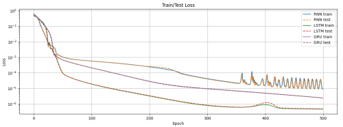
We run the script to compare the performance, and the results are as follows:
-
Loss curves of the three models:
-
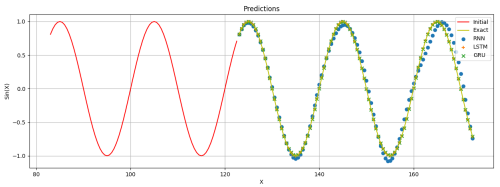
Predictions of the three models:
The compare_results.py script runs the RNN, LSTM, and GRU models in turn. If I run it on my computer with a GPU (NVIDIA GeForce GTX 4060 Ti), it takes about 30 seconds, with a maximum memory usage of about 354 MB. If I run it on a CPU (Intel i5-9600K), it takes about 3 minutes and 33 seconds.
I have run this comparison performance script multiple times, and the results vary each time. In most cases, all three models can fit the sine function sequence data well, but overall, LSTM and GRU perform slightly better than RNN.
Summary
In this article, we introduced the working principles of Gated Recurrent Unit (GRU) and Long Short-Term Memory (LSTM) and implemented these two models using PyTorch. We used these two models to predict the sine function sequence data and compared them with a simple Recurrent Neural Network (RNN). We found that LSTM and GRU perform better than RNN in capturing long-term dependencies in sequence data, thus improving the model’s performance.