Background
This is the fourth article in the “Learn PyTorch by Examples” series. In the previous three articles:
- “Learn PyTorch by Example (1): PyTorch Basics and MNIST Handwritten Digit Recognition (I)”
- “Learn PyTorch by Example (2): Parameter Selection in MNIST Handwritten Digit Recognition (II)”
- “Learn PyTorch by Example (3): MNIST Handwritten Digit Recognition with Convolutional Neural Networks (III)”
In the articles, we introduced how to solve image classification problems using PyTorch. Another important problem in machine learning is sequence prediction. Unlike image classification, sequence prediction requires considering the correlation between data. Recurrent Neural Network (RNN) is a neural network that can handle sequence data, as it saves the previous data information at each time step. In this article, we will use a simple RNN to predict the sine function.
There is an example in the PyTorch official repository https://github.com/pytorch/examples/, which uses Long Short-Term Memory (LSTM) to predict the sine function. We will not consider LSTM for now, but use a simple RNN to predict the sine function.
The code for this article can be found in the T04_series_rnn folder in my GitHub repository https://github.com/jin-li/pytorch-tutorial.
Recurrent Neural Network (RNN) Introduction
In the previous articles, we introduced feedforward neural networks, including fully connected neural networks and convolutional neural networks. Both of them are feedforward neural networks. A disadvantage of feedforward neural networks is that they cannot handle sequence data because they do not store previous data information. Recurrent Neural Network (RNN) is a neural network that can handle sequence data. It saves the previous data information at each time step, so it can handle sequence data. It is worth noting that the sequence data here is not necessarily time series data, but can also be spatial sequence data. For example, sentences in natural language processing are spatial sequence data, and audio data in speech recognition is sequence data. For convenience, we call each element in the sequence a time step.
The structure of RNN is not complicated. Its core has two points:
- During training, the training data needs to be unfolded according to time steps, and then the loss function is calculated by traversing each time step. Finally, the weights are updated through the backpropagation algorithm.
- For each time step, there is not only an output but also a hidden state. This hidden state is passed to the next time step, thus retaining the previous data information.
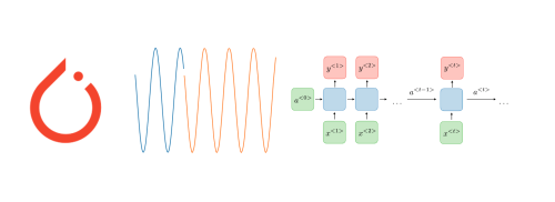
For more information about RNN, you can refer to the CS230 course slides from Stanford University. Here we use an animated image to briefly illustrate how RNN works:
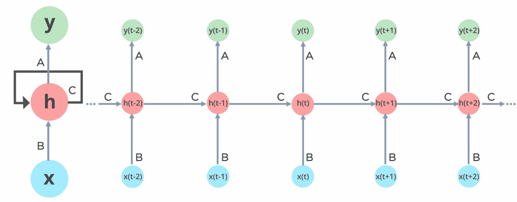
Here, $x$ is the input, $h$ is the hidden state, $y$ is the output, and $t$ is the time step. It can be seen that the hidden state $h$ is passed to the next time step at each time step, thus retaining the previous data information. $x$, $h$, and $y$ are each a layer of the neural network. $h$ is the hidden layer, $x$ is the input layer, and $y$ is the output layer. The size of each layer can be determined according to the specific problem.
Sine Function Prediction
The sine function can be regarded as a time series. At some moments, the value of the sine function may be the same, but the values after that may be different. For example, for $y = \sin(x)$, when $x = 0$ and $x = \pi$, $y$ is both $0$, but at the next time step of these two moments (assuming the time step size is 0.01, then the next two time steps are $x = 0.01$ and $x = \pi + 0.01$), $y$ is different. To predict the value of the next time step, we need to know not only the value of the current time step but also the values of the previous several time steps. This is exactly the purpose of the Recurrent Neural Network.
RNN Model Design
This problem is relatively simple, and we only need to use a Recurrent Neural Network. The input of our Recurrent Neural Network is a sequence, and the output is the next value of this sequence. The input sequence is the value of the sine function, and the output is the next value of the sine function. The structure of our Recurrent Neural Network is as follows:
- Input layer: The size of the input layer is 1, that is, there is only one input at each time step.
- Hidden layer: The size of the hidden layer can be chosen arbitrarily. Considering that this problem is relatively simple, we choose 10 neurons as the hidden layer.
- Output layer: The size of the output layer is 1, that is, there is only one output at each time step.
In this way, the structure of our Recurrent Neural Network is determined. We can use the nn.RNN class in PyTorch to implement this Recurrent Neural Network:
|
|
Here we define a SimpleRNN class, which inherits from PyTorch’s nn.Module class. In the __init__ function, we define an instance of the nn.RNN class, which is our Recurrent Neural Network. In the forward function, we define the forward propagation process of the Recurrent Neural Network, that is, how we calculate the output. Here we only need to return the output of the last time step.
Data Preparation
In the previous three articles, we used datasets that others had prepared when training neural networks. But here, we need to prepare the data ourselves. For this problem, data preparation is very simple. We only need to generate some sine function data. After generating the data, we need to encapsulate it into a PyTorch Dataset class so that we can easily load the data using PyTorch’s DataLoader class.
The complete code for generating the dataset can be found in the SineWaveDataset.py file in the T04_series_rnn folder in the GitHub repository corresponding to this article https://github.com/jin-li/pytorch-tutorial. The specific code is as follows:
|
|
- First, we define an
RNNDatasetclass to store the training data. It inherits from PyTorch’sDatasetclass so that we can use PyTorch’sDataLoaderclass to load the data. - Then we define a
create_datasetfunction to generate the sine function data. This function has two input parameters. One issequence_length, which indicates how many time steps of data we use to predict the next time step of data. The other istrain_percent, which indicates how much of the data we use for training, and the rest is used for testing. The main work of this function is to generate the sine function data and encapsulate it into an instance of theRNNDatasetclass. Finally, we save the training data and test data to the filestrain_data.ptandtest_data.pt. - In the
create_datasetfunction, we first generate 2000 time steps of sine function data. Then we generate some sequence data for training from this sine data. The method of generating training data is:- Starting from the first time step, take 50 consecutive time steps of data as a sequence, i.e., $x_1, x_2, \cdots, x_{80}$.
- The next time step after these 50 time steps is the value to be predicted, $y = x_{81}$.
- Repeat the above process until all time steps are taken. Here we have 2000 time steps, so we can generate a total of $2000 - 80 = 1920$ sequences.
- We divide these 1950 sequence data into two parts, 80% for training ($1920 \times 0.8 = 1536$) and 20% for testing.
- Finally, we encapsulate the training data and test data into instances of the
RNNDatasetclass and save them to the filestrain_data.ptandtest_data.pt.x_trainis a 3-D tensor with a size of $1536 \times 80 \times 1$, where $1536$ is the number of training samples, $80$ is the sequence length, and $1$ is the input size.y_trainis a 2-D tensor with a size of $1536 \times 1$, where $1536$ is the number of training samples, and $1$ is the output size.
Model Training
As in the previous articles, we need to define a training function to train our model. The code for this training function is also simple:
|
|
The input parameters of this training function are similar to the training function in the previous articles, namely the model, training data loader, loss function, and optimizer, which are not repeated here.
Model Testing
In addition to the training function, we define a testing function. After training an epoch, we need to test the performance of our model on the test data. The code for the testing function is as follows:
|
|
Model Prediction
Finally, we define a prediction function to test whether our model can predict the values of a sine function sequence based on a given sequence of data. The code for the prediction function is as follows:
|
|
Run the Model
We integrate the above code into one file and call the above functions in the main() function. As before, we add some command-line parameters to control the training and testing of the model. The complete code can be found in the T04_series_rnn folder in my GitHub repository https://github.com/jin-li/pytorch-tutorial, in the time_series_rnn.py file.
-
First, we generate the sine function dataset:
1python SineWaveDataset.py -
Then we train the model, use the model to predict a sine function sequence, and plot the prediction results with the true results:
1python time_series_rnn.py --plotThis code runs for about 20 seconds on the GPU, with a memory usage of about 208M; if using the CPU, the running time increases to about 1 minute and 30 seconds. After running this command, we can see the model prediction results as shown in the figure below:
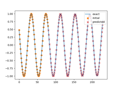
The first 80 data points are an initial sequence, and the next 150 data points are the model’s prediction results. It can be seen that the model’s prediction results are very close to the true results.
Summary
In this article, we introduced how to use PyTorch to implement a simple Recurrent Neural Network (RNN) to predict a sine function sequence.
In this article, I ran the example with different random seeds multiple times. The results shown above are from one of the runs with a random seed of 18 (the default value in the code on GitHub). Readers can adjust the model parameters according to the parameter selection method we introduced in the second article of this series “Learn PyTorch by Example (2): Parameter Selection in MNIST Handwritten Digit Recognition (II)” to see if they can get better results.
With this simple example as a foundation, we will introduce how to use other neural networks, such as Long Short-Term Memory (LSTM), Gated Recurrent Unit (GRU), etc., to predict the sine function sequence in the next article.